Abstract

In this second part, we focus entirely on the transport layer, the level at which reliability, ordering, congestion control, and latency behavior are determined.

While higher-level libraries abstract networking into simple read and write calls, the true performance characteristics of a trading system are dictated by the mechanics of TCP and UDP. Understanding how these protocols behave under load, packet loss, congestion, and burst traffic is essential for anyone building low-latency infrastructure.

We will analyze TCP in depth, including connection lifecycle, three-way handshake, sequence numbers, acknowledgements, retransmission logic, sliding windows, congestion control algorithms, flow control, head-of-line blocking, and the impact of mechanisms such as Nagle’s algorithm and delayed acknowledgements. We will examine how TCP reacts to packet loss and why retransmissions directly affect latency stability.

We will then study UDP, its connectionless nature, absence of reliability guarantees, lack of congestion control, and why it is often preferred for market data distribution in trading systems. We will discuss what must be implemented at the application layer when using UDP, including sequencing, gap detection, and replay mechanisms.

Throughout this part, we will connect protocol mechanics to real-world trading infrastructure decisions. We will explain why order flow typically uses TCP while market data frequently uses UDP, and we will highlight the types of transport-layer questions that are commonly asked in quantitative developer and market-making interviews.

This section aims to move beyond surface-level protocol knowledge and provide a systems-level understanding of how transport-layer behavior directly influences determinism, throughput, and profitability in modern electronic markets.

Part 1: Networking basics
Part 2: TCP and UDP in trading systems
Part 3: WebSocket implementation

TCP – Reliability, Ordering, and Control

If IP is responsible for moving packets across networks, TCP is responsible for turning that unreliable packet delivery into a reliable, ordered byte stream between two processes. When you submit an order to an exchange over a WebSocket connection, TCP is the protocol that guarantees that the bytes representing your order will arrive, in order, without corruption, or that you will be informed if the connection has failed.

That guarantee is not trivial. It is implemented through a complex state machine inside the operating system kernel. To understand TCP properly, we must examine its lifecycle, its reliability model, and its control mechanisms.

Connection Lifecycle

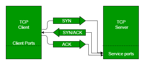
TCP is connection-oriented. Before any data is exchanged, both sides must synchronize state. This begins with the three-way handshake.

The client initiates the connection by sending a SYN packet. This packet contains an initial sequence number. The sequence number is not arbitrary. It is the starting point for numbering every byte that will be sent during the connection. The server replies with a SYN-ACK. This packet acknowledges the client’s initial sequence number and provides the server’s own initial sequence number. Finally, the client responds with an ACK. At this moment:

• Both sides know the other’s starting sequence number.
• Both sides confirm bidirectional reachability.
• The connection transitions to the ESTABLISHED state.

The handshake serves two fundamental purposes.

First, it confirms that packets can travel in both directions. Second, it synchronizes sequence number spaces so that every byte transmitted can be tracked precisely. In a trading context, this handshake represents the moment a session becomes transport-level active. Any latency here directly contributes to connection setup time, which matters during reconnect scenarios.

Sequence Numbers

TCP does not track packets. It tracks bytes. Every byte transmitted in a TCP connection is assigned a sequence number. If a segment contains 1000 bytes starting at sequence number 5000, the next expected byte after successful delivery is 6000.

The receiver does not acknowledge individual packets. It acknowledges the next byte it expects to receive.

For example, if the receiver sends ACK 6000, it means that it has received all bytes up to 5999 successfully.
This cumulative acknowledgement mechanism simplifies recovery but introduces important behavior under packet loss.

Reliability Through Retransmission

TCP assumes that packet loss is possible. The internet does not guarantee delivery. If a segment is lost:

• The receiver continues acknowledging the last contiguous byte received.
• The sender notices repeated duplicate acknowledgements.
• After receiving a threshold number of duplicate ACKs, the sender triggers a fast retransmit.
• Alternatively, if acknowledgements stop entirely, a retransmission timeout occurs.

When retransmission happens, the lost segment is sent again. This mechanism ensures reliability, however, retransmission is not free. It increases latency and may reduce throughput because TCP interprets loss as a signal of congestion.

In a low-latency trading system, packet loss translates directly into unpredictable latency spikes.

Example

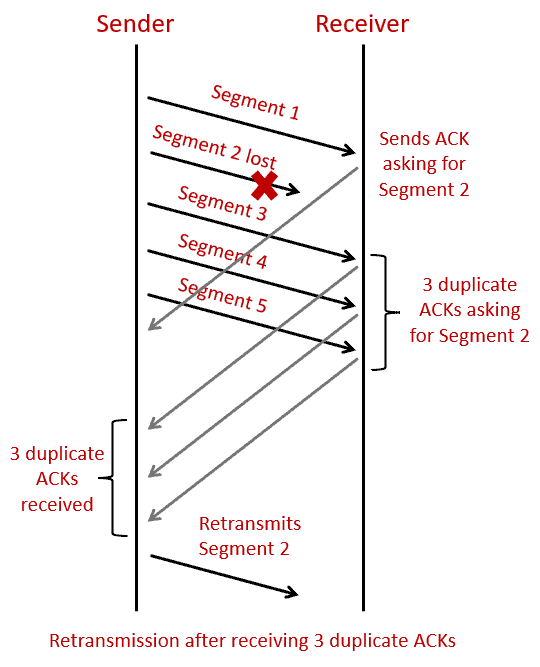
Once the retransmitted Segment 2 arrives, the receiver can deliver all buffered data in order and send a cumulative acknowledgement confirming successful receipt. This mechanism allows TCP to recover from packet loss quickly, but it still introduces latency and typically reduces the congestion window, affecting short-term throughput.

Sliding Window

TCP does not send data one segment at a time and wait for acknowledgement. That would be inefficient. Instead, it uses a sliding window mechanism. This allows multiple segments to be “in flight” simultaneously. There are two distinct windows involved.

Flow Control Window

Congestion Window

The receiver advertises how much buffer space it has available. This is known as the receive window. If the application on the receiving side is slow to consume data, the receive buffer fills. The advertised window shrinks. Eventually, it may reach zero. When that happens, the sender must stop transmitting new data until the window reopens. Flow control protects the receiving process from being overwhelmed.

The congestion window is maintained by the sender and reflects its estimate of how much data the network can handle without becoming congested. TCP uses algorithms such as: Slow Start, Congestion Avoidance, Fast Retransmit, Fast Recovery, CUBIC

At the beginning of a connection, TCP starts conservatively. It gradually increases its sending rate until it detects packet loss. When loss occurs, TCP reduces its congestion window and slows down. This behavior ensures network stability, but it introduces variability in throughput and latency.

In trading environments where deterministic behavior is valued, congestion control dynamics can impact performance under burst traffic or transient loss.

Head-of-Line Blocking

One of the most important characteristics of TCP is that it guarantees ordered delivery. If segment number N is lost, but segments N+1 and N+2 arrive successfully:

• TCP buffers N+1 and N+2.
• The application receives nothing.
• Delivery stalls until N is retransmitted.

This is head-of-line blocking. It ensures correctness and ordering, but it also means that a single lost packet can temporarily freeze an entire stream. and this could be unacceptable for certain applications!

For order submission, this is acceptable. Missing or reordering an order is catastrophic. For market data, this can be problematic. If real-time price updates stall because of a single lost packet, the trading strategy may operate on stale data.
This is one of the primary reasons why market data feeds are often distributed using UDP.

Latency vs Efficiency

By default, TCP may attempt to reduce network overhead by merging small writes into larger segments. If small chunks of data are written rapidly, TCP may delay sending them until either:

• Enough data accumulates to fill a segment.
• An acknowledgement is received.

This is known as Nagle’s algorithm. It improves bandwidth efficiency but introduces delay.

In high-frequency trading systems, even microsecond-level delays can be undesirable. Therefore, TCP_NODELAY is often enabled to disable Nagle’s algorithm and force immediate transmission of small messages.

Keepalive and Application Heartbeats

TCP includes an optional keepalive mechanism implemented inside the operating system kernel. Its purpose is simple: detect whether the remote peer is still reachable at the transport level when a connection has been idle for a long time.

If enabled, TCP keepalive works as follows:

• After a long period of inactivity, the kernel sends a small probe packet to the peer
  • If the peer responds with an acknowledgement, the connection is considered alive
  • If multiple probes go unanswered, the kernel eventually declares the connection dead and closes it

There are two important characteristics of TCP keepalive.

• Operates purely at the transport layer. It does not understand application protocols, sessions, authentication, or business logic. It only verifies that the remote TCP stack is still responding.
• Default timers are usually very long. On many systems, keepalive may only trigger after hours of inactivity unless explicitly reconfigured. This makes it unsuitable as a primary liveness detection mechanism in trading systems, where seconds matter.

Now let’s analyze the alternative application-layer heartbeats.

Exchanges typically define their own heartbeat mechanism within the application protocol. For example, a WebSocket API may require periodic ping messages, or a FIX session may require heartbeat messages at a negotiated interval. Application heartbeats serve a different purpose. They verify logical session liveness, not just transport reachability. A TCP connection may be technically established and responsive at the kernel level, but the exchange session may be invalid due to:

• Missed authentication
• Internal exchange restart
• Session timeout policies
• Logical protocol errors

In such cases, TCP keepalive would still report the connection as alive because packets can still be exchanged at the transport layer. However, the trading session is effectively dead from a business perspective. Application heartbeats detect these conditions. If the exchange does not receive required pings within a specified interval, it may terminate the session. If the client does not receive expected heartbeat responses, it can proactively reconnect.

A connection can be alive at the TCP level but unusable at the trading protocol level. Robust systems monitor both.

Congestion Algorithm – Cubic

CUBIC is a loss-based TCP congestion control algorithm designed to perform efficiently in high-bandwidth, high-latency networks where traditional Reno-style TCP becomes too conservative and slow to recover.

To understand CUBIC, first recall how Reno behaves. After a congestion event, Reno halves the congestion window and then increases it linearly, roughly one MSS (Maximum Segment Size) per RTT (Round-Trip Time). This makes recovery directly dependent on round-trip time. In networks with large bandwidth-delay products, the optimal congestion window may be very large, and linear growth can take a long time to return to full throughput. As a result, Reno underutilizes available bandwidth in modern high-speed links.

CUBIC changes the growth model fundamentally. Instead of increasing the congestion window based on acknowledgements, it increases it as a function of elapsed time since the last congestion event. The window evolves according to a cubic function:

Here, t is the time since the last window reduction, W_{max} is the window size just before the last congestion event, C is a scaling constant, and K determines the inflection point of the curve. Conceptually, this means that window growth is slow immediately after a loss, then accelerates, then flattens as it approaches the previous maximum window size.

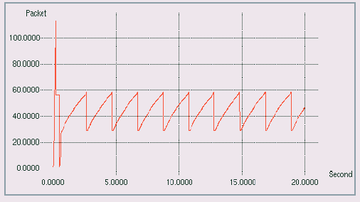
The graph you provided reflects exactly this behavior. After slow start, the congestion window drops when a loss is detected. Instead of rising linearly as in Reno, it follows a smooth cubic curve. Near the previous maximum window, the curve becomes flatter. This creates a plateau where the algorithm gently probes around the prior congestion point instead of aggressively overshooting it. If no new loss occurs, the curve steepens again and probes for additional bandwidth beyond the previous maximum.

When congestion is detected, CUBIC still applies a multiplicative decrease similar to Reno, but typically less aggressively. The new window is often computed as:

with \beta commonly around 0.7 rather than Reno’s 0.5. This softer reduction allows faster recovery while still reacting conservatively to congestion.

One of the most important properties of CUBIC is that its growth depends on time rather than RTT. Because the window increases according to elapsed time since the last loss, flows with different round-trip times tend to grow more fairly compared to Reno, where shorter RTT flows increase faster. This makes CUBIC particularly suitable for long-distance, high-speed links.

However, CUBIC remains fundamentally loss-based. Packet loss is still interpreted as a signal of congestion. When loss occurs, the congestion window is reduced and the cubic growth cycle restarts. In latency-sensitive systems, this still introduces variability: retransmissions occur, the window shrinks, and throughput temporarily drops.

In essence, CUBIC transforms TCP congestion control from a linear, ACK-driven process into a smooth, time-driven cubic control system. It recovers large windows faster, reduces RTT bias, and better utilizes modern high-capacity networks, which is why it became the default congestion control algorithm in Linux.

UDP – Simplicity, Latency and Responsibility

If TCP is about reliability, ordering, and congestion control, UDP is about minimalism. UDP (User Datagram Protocol) sits at the transport layer just like TCP, but it removes almost all of the machinery that makes TCP complex. There is no connection handshake. There is no sequence tracking. There are no acknowledgements, no retransmissions, no congestion window, and no flow control. UDP provides only one essential service: it delivers discrete datagrams from one process to another.

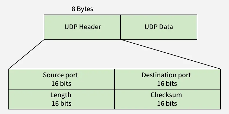
A UDP packet contains a small header with a source port, destination port, length field, and checksum. That is all. Once the application hands data to the kernel via a UDP socket, the kernel wraps it in a UDP header, then in an IP packet, and sends it. There is no guarantee that it will arrive. There is no guarantee that it will arrive once. There is no guarantee that it will arrive in order.

UDP preserves message boundaries. If you send 200 bytes in one call, the receiver gets exactly one 200-byte datagram, or nothing at all. This is fundamentally different from TCP, which provides a continuous byte stream with no inherent message boundaries.

Because UDP is connectionless, there is no handshake phase. A client can send data immediately. The operating system does not maintain per-connection state machines like TCP’s SYN_SENT or ESTABLISHED. This dramatically reduces overhead and complexity inside the kernel. It also reduces latency, especially in burst scenarios.

However, the simplicity of UDP shifts responsibility upward. If reliability is required, the application must implement it. That may include:

• Adding sequence numbers to detect missing messages
• Implementing gap detection logic
• Requesting retransmission from a replay server
• Maintaining its own ordering guarantees
• Implementing rate control

In trading systems, this trade-off is intentional.

Market data feeds are frequently distributed over UDP, often via multicast. The reasoning is straightforward. Market data is high volume and continuous. If one update is lost, the next update may contain sufficient state to recover. It is better to lose a single price update than to stall the entire stream waiting for retransmission, as would happen with TCP due to head-of-line blocking.

For example, suppose a price feed sends updates 101, 102, 103, and packet 102 is lost. With UDP, the application detects a gap in sequence numbers and may request a replay, but it can continue processing 103 immediately. With TCP, delivery would stall at 102 until retransmission completes. This difference is crucial in low-latency environments.

UDP also avoids congestion control at the transport layer. It does not reduce sending rate when loss occurs. This makes it potentially dangerous on shared networks, because it can contribute to congestion collapse if misused. In controlled environments such as exchange multicast networks or colocated data centers, infrastructure-level traffic shaping is often used instead of relying on TCP’s built-in congestion control.

IP Fragmentation

One of the most subtle and dangerous aspects of UDP is its interaction with the Maximum Transmission Unit, or MTU. At first glance, UDP appears simple: the application sends a datagram, and the receiver receives that same datagram as a single unit. Unlike TCP, UDP preserves message boundaries. If you send 1200 bytes in one call, the receiver obtains exactly one 1200-byte message. However, that simplicity hides an important constraint imposed by the lower layers of the network stack!

In most Ethernet networks, the MTU is 1500 bytes. This means that the maximum size of an IP packet payload that can fit inside a single Ethernet frame is 1500 bytes. But this 1500 bytes must include not only application data, but also protocol headers. For IPv4, the IP header is typically 20 bytes, and the UDP header is 8 bytes. This leaves approximately 1472 bytes available for actual UDP payload if fragmentation is to be avoided. If a UDP datagram exceeds this size, the IP layer is forced to fragment it.

Fragmentation occurs below the transport layer. The large IP packet is split into multiple smaller IP fragments, each with its own IP header and offset information. These fragments travel independently across the network. At the destination, the IP layer attempts to reassemble them into the original datagram before passing it up to UDP.
The crucial point is that reassembly is all-or-nothing. If even a single fragment is lost, the entire UDP datagram is discarded. There is no partial recovery. There is no retransmission at the UDP layer. From the perspective of the receiving application, the message simply never arrives. This dramatically increases effective loss probability.

Suppose a large UDP message is split into three fragments. Even if each fragment has only a small probability of loss, the probability that all fragments arrive successfully is the product (assuming that events are independent) of their individual success probabilities. As the number of fragments increases, the overall probability of successful reassembly decreases rapidly. In other words, fragmentation amplifies packet loss risk. In latency-sensitive systems, this is unacceptable.

Market data feeds in trading environments are therefore carefully engineered to fit within a single MTU-sized packet. Exchanges typically ensure that multicast packets remain comfortably below the fragmentation threshold. Sending a fragmented UDP packet in a low-latency trading system is often considered a design error.

Fragmentation also introduces latency. The receiver cannot process the datagram until all fragments arrive and are reassembled. This adds variability and complicates performance predictability. Furthermore, diagnosing fragmentation-related issues in production environments can be difficult, especially across WAN links where intermediate routers may have smaller MTUs than expected.

Across long-distance or heterogeneous networks, Path MTU Discovery is used to determine the smallest MTU along the route. If this mechanism fails or is misconfigured, fragmentation may occur unpredictably. For systems that demand deterministic latency behavior, such unpredictability is a serious concern. The key insight is this: UDP does not protect you from lower-layer constraints. It will happily accept a large payload and pass it down the stack. It is the responsibility of the system designer to ensure that datagrams remain within safe size limits.

Socket Buffers and Silent Packet Drops

Unlike TCP, UDP provides no flow control and no congestion control at the transport layer. This simplicity removes overhead and reduces latency, but it also means that the kernel does not protect the receiving application from overload. When using UDP, the responsibility for keeping up with incoming traffic shifts almost entirely to the application and the surrounding system architecture.

When a UDP packet arrives at the network interface card, it is placed into a receive queue managed by the kernel. From there, it is copied into the UDP socket’s receive buffer. This buffer is finite and its size is controlled by system parameters and can be tuned, but it is never infinite. If the application reads from the socket quickly enough, the buffer remains healthy. Packets arrive, are copied into the buffer, and are promptly consumed. However, if the application falls behind, for example due to CPU contention, garbage collection pauses, locking contention, or heavy computation, the receive buffer begins to fill.

Once the receive buffer is full, new incoming UDP packets are simply dropped. The packets disappear silently at the kernel level.

• There is no retransmission request.
• There is no backpressure signal.
• There is no congestion window reduction.
• There is no error returned to the sender.

This is one of the most important operational realities of UDP in trading systems. Loss does not necessarily mean the network dropped the packet. The kernel may have dropped it locally because the application could not keep up.

In high-throughput market data systems, this becomes critical. A burst of messages, for example during a volatility spike, can temporarily exceed the processing capacity of the application. If socket buffers are undersized or processing pipelines are inefficient, packet drops will occur even on a perfectly healthy network. From the application’s perspective, the only observable symptom may be a gap in sequence numbers embedded in the feed. That gap might be incorrectly attributed to “network loss,” when in reality it was caused by local buffer overflow.

Because UDP does not implement flow control, the sender will continue transmitting at full rate regardless of the receiver’s state. There is no automatic throttling. If the receiver is overwhelmed, loss is inevitable. This is fundamentally different from TCP. In TCP, the receiver advertises a receive window, and the sender adjusts its transmission rate accordingly. In UDP, there is no such mechanism. The transport layer provides no protection.

This is the trade-off: UDP eliminates head-of-line blocking and retransmission delay, but it also eliminates built-in safety mechanisms. In high-performance trading infrastructure, maintaining stability under burst load requires deep understanding of kernel buffers, interrupt handling, CPU scheduling, and application-level sequencing.

Multicast

So far we have discussed UDP in the context of point-to-point communication, where one sender transmits datagrams to one receiver. In real trading infrastructure, however, market data is rarely distributed using simple unicast. Instead, exchanges and data vendors typically rely on UDP multicast. Multicast is fundamentally different from unicast. In unicast communication, the sender must transmit one copy of each packet per receiver. If 100 trading firms subscribe to the same market data feed over unicast, the exchange must send 100 identical packets. This creates unnecessary duplication and network overhead.

With multicast, the sender transmits a single packet, and the network infrastructure replicates it only where necessary. Switches and routers forward multicast packets to all subscribers that have explicitly joined the multicast group. This allows one-to-many distribution without duplicating traffic at the source. This model is extremely efficient and is one of the main reasons UDP is preferred for market data sharing.

How Multicast Works

Multicast uses special IP address ranges reserved for group communication. A sender transmits packets to a multicast IP address rather than to a specific host. Receivers that want to receive the stream must explicitly join that multicast group. Group membership is managed using IGMP (Internet Group Management Protocol). When a trading server subscribes to a feed, it informs the local router or switch that it wants to receive traffic for that multicast group. The network infrastructure then ensures that multicast packets are forwarded only to interfaces with active subscribers. Importantly:

• The sender does not maintain per-client state.
• There is no handshake.
• There is no awareness of how many receivers exist.
• The sender simply transmits to the group address.

This makes multicast highly scalable!

Why Multicast Is Ideal for Market Data

Market data has very specific characteristics:

• High throughput
• Continuous stream
• Many simultaneous consumers
• Identical content for all participants

Multicast aligns perfectly with these requirements. If an exchange publishes a price update, every subscriber should see the same message at roughly the same time. Sending a single multicast packet ensures minimal duplication and consistent timing across receivers.

Because UDP is connectionless and does not require acknowledgements, the exchange can transmit updates at extremely high rates without being slowed down by individual receiver behavior. Latency remains predictable as long as the network is not congested.

The Trade-Off

Multicast provides no delivery guarantees. If a packet is lost anywhere along the path, that subscriber simply misses it. The sender does not know, and it does not care. Therefore, market data protocols implement recovery mechanisms at the application layer:

• Sequence numbers embedded in each packet
• Gap detection by subscribers
• Replay servers for missing data
• Snapshot recovery mechanisms

The real-time feed is delivered via UDP multicast for speed. Recovery is handled separately and only when necessary. This design minimizes latency for the normal case while still allowing state consistency to be restored when loss occurs.