Reconstructing the Full Order Book with Deribit WebSocket Client
Abstract
While working on my C++ Deribit WebSocket client, I recently added a feature that allows the program to maintain and monitor the full order book in real time, an essential feature for a trading strategy. The goal was to build a local representation of the market that stays synchronized with the exchange and can be used to analyze liquidity, spreads, and short term supply and demand dynamics.
The Deribit WebSocket API provides incremental updates of the order book rather than full snapshots at every update. This means that the client must reconstruct the state of the book locally by applying each update as it arrives. Implementing this correctly requires careful handling of price levels, update ordering, and internal data structures so that the local view always reflects the latest exchange state. This feature is now integrated directly into my client, which is available in my GitHub repository. The order book is updated continuously and the client exposes useful quantities such as best bid and ask prices, mid price, spread, and liquidity across multiple levels of the book.
In addition to implementing the order book monitoring, I also ran a small latency analysis on the feed. The measurements were taken from a home environment using a Starlink connection under load, so they should not be interpreted as precise infrastructure measurements. Still, the experiment provided an interesting look at the distribution of market data delays and served as a simple validation of the timestamp pipeline in the client.
Reconstructing the Order Book
The Deribit market data feed does not continuously send the full order book. Instead, it provides incremental updates that describe how individual price levels change over time. To maintain a consistent view of the market, the client must reconstruct the order book locally by applying these updates as they arrive. The client subscribes to the WebSocket channel:
"book.<instrument>.<type>"The interval parameter defines how frequently updates are sent. According to the Deribit API, events are aggregated over the specified interval before being delivered to the client. The available values are {“raw”, “100ms”, “agg2”}.
The raw stream sends updates without aggregation. In this implementation I used the 100ms interval, which means that order book changes are grouped and delivered roughly every 100 milliseconds.
Each message contains modifications to specific price levels on both sides of the book. A price level can appear, change size, or disappear depending on how the underlying orders evolve on the exchange. Internally, the client maintains two ordered structures representing the bid and ask sides of the book. When an update arrives, the message is parsed and the affected levels are applied to the local structures. If the quantity at a price becomes zero, the level is removed from the book. If a new level appears, it is inserted in the correct position.
Because the updates are incremental, the client continuously evolves the current state of the book rather than rebuilding it from scratch. This allows the program to maintain a synchronized representation of the exchange order book with minimal processing overhead. Once the book is updated, the client can immediately compute quantities such as the best bid, best ask, mid price, and spread. It can also aggregate liquidity across multiple levels and evaluate order book imbalance.
The animation below shows how the reconstructed book evolves over time as updates arrive from the exchange.
Visualizing Order Book Liquidity
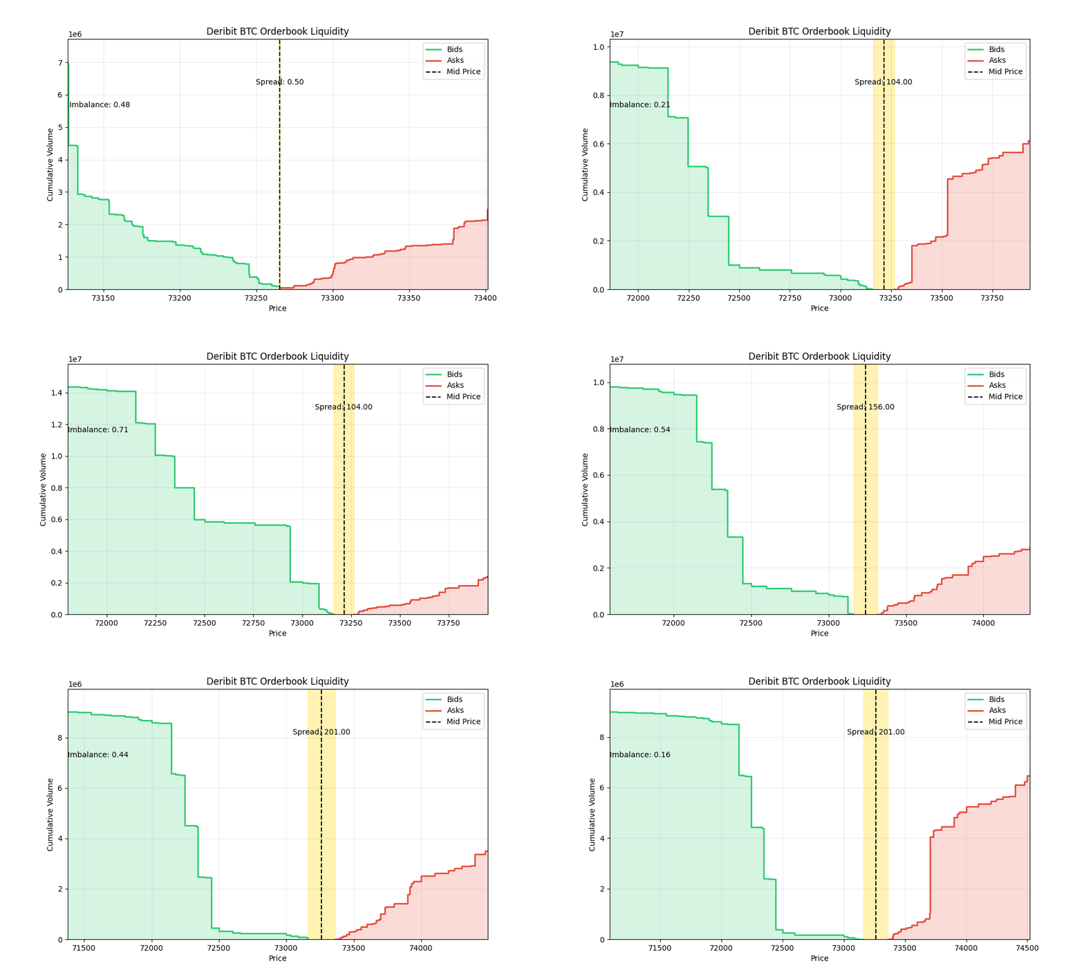
Once the local order book is reconstructed, it becomes possible to analyze the structure of liquidity around the current market price. A simple way to represent this is through a depth chart, which shows the cumulative volume available on the bid and ask sides of the book.
In this representation the horizontal axis shows the price levels, while the vertical axis shows the cumulative volume available at or better than that price. The green curve represents the bid side of the order book. As the price moves further away from the mid price, the curve increases because it accumulates the total quantity of buy orders resting in the book. The red curve represents the ask side, which accumulates the total volume of sell orders.
The dashed vertical line indicates the mid price, which is computed as the average between the best bid and best ask. The highlighted band around it marks the spread, which in this snapshot is approximately 201 dollars.
Spread(t) = Ask_{best}(t) - Bid_{best}(t) Another useful metric visible in the chart is the order book imbalance. In this example the imbalance is close to 0.50, which suggests that the liquidity on the bid and ask sides is relatively balanced near the mid price. In other situations this value can shift noticeably, indicating that one side of the book is heavier than the other.
Imbalance(t) = \frac{Bid_{volume}(t) }{Bid_{volume}(t) + Ask_{volume}(t) }Visualizations like this make it easier to understand how liquidity is distributed around the market price. Even though the raw order book consists of many discrete price levels, the cumulative representation reveals the overall shape of the supply and demand curves implied by the resting orders.
Measuring Feed Latency
While working with the order book stream, I also ran a small experiment to observe the latency of the market data feed. The goal was not to obtain precise infrastructure measurements, but simply to understand how long it takes for order book updates generated by the exchange to reach the client. Each update sent by Deribit includes a timestamp produced by the exchange. When a message arrives through the WebSocket connection, the client records a second timestamp using the local system clock. The difference between the two provides a simple estimate of the feed latency. The latency for each update can therefore be approximated as:
Latency = t_{receive} - t_{exchange}where the first term represents the time at which the client receives the message and the second term corresponds to the timestamp generated by the exchange. This measurement captures several components of delay, including exchange processing, message aggregation, network transmission, and client side processing.
Latency Distribution
The histogram below shows the distribution of measured latencies for the collected sample of order book updates.

Most updates arrive within a relatively narrow range. The median latency is approximately 55 milliseconds, while the higher percentiles extend further into the tail of the distribution. The summary statistics from the sample are:
| Metric | Latency |
|---|---|
| p50 | 55 ms |
| p90 | 124 ms |
| p99 | 166 ms |
The long tail visible in the histogram indicates that occasional spikes occur, which is common in real time data streams. These spikes can be caused by temporary network congestion, batching of updates by the exchange, or scheduling delays on the client side.
Latency Over Time
Another way to examine the behavior of the feed is to look at latency as a function of the sequence of received updates.

The time series shows that most updates cluster around the median latency, while occasional spikes appear throughout the sample. These spikes correspond to the high latency values observed in the tail of the distribution. Despite these fluctuations, the baseline latency remains relatively stable across the entire observation window.
Estimating the Network Contribution
To separate the network component from the overall delay, I performed a simple ping measurement to estimate the round trip time between the client and the Deribit servers. The minimum round trip time (RTT) was used to approximate the lower bound of the network delay. Since a ping measures a round trip, the one way latency can be approximated as:
Network\ Latency \approx \frac{RTT_{min}}{2}Subtracting this estimate from the raw feed latency provides a rough indication of the portion of delay that may originate from exchange side processing and message aggregation. The comparison between the two distributions is shown below.

After removing the estimated network component, the median latency decreases from about 55 ms to roughly 40 ms, suggesting that a significant fraction of the observed delay is attributable to network transmission.
Notes on the Measurement
These measurements should be interpreted cautiously. The test was performed from a home environment using a Starlink connection that was under load, and the system clocks were not synchronized with the exchange clock. For this reason the experiment should be viewed mainly as a sanity check of the data pipeline rather than an accurate measurement of exchange infrastructure latency. Still, it provides an interesting glimpse into how market data arrives in practice and highlights the variability that can occur even in relatively stable network conditions.
Leave a Reply