A Gurobi-based hedging engine in Python

In this project, developed as part of the Robust Optimization course at Polytechnic of Turin, I built a small but complete risk-management engine that optimizes how a company hedges a future foreign-currency payment using forward contracts and call options.
The code is fully implemented in Python, with Gurobi as the optimization backend, and is publicly available in my GitHub repository “RiskManagement”.

The goal of this article is twofold:

• Explain the financial logic behind the models (VaR / CVaR, forwards, options, distributional uncertainty).
• Show the quantitative and engineering skills behind the code, including mathematical modeling, mixed-integer optimization, and distributionally robust optimization (DRO).

Problem setup: hedging a future FX payment

Consider a firm that must buy a given amount of foreign currency (say USD) at a future date T. The home currency is, for example, EUR. The main risk is that the EUR/USD spot rate at T moves unfavorably.

The project assumes that the firm can combine:

• Forward contracts: commit today to buy foreign currency at T at a fixed forward rate F.
• Call options: pay a premium today for the right, but not the obligation, to buy foreign currency at T at strike K_i.

To stress-test the strategy, I model three macro scenarios with different domestic and foreign interest rates, corresponding to strong, neutral and weak USD environments. (GitHub)

Formally, let \mathcal S be the set of scenarios, each with probability \pi_s and terminal spot S_T^s. The company must cover a notional foreign exposure Q (e.g., the number of USD to purchase at T).

Risk measure: from VaR to CVaR

The project focuses on Value-at-Risk (VaR) and Conditional Value-at-Risk (CVaR) as key risk measures.

• For a loss random variable L, the \alpha-VaR is

\operatorname{VaR}_\alpha(L) = \inf{ \eta \in \mathbb R : \mathbb P(L \le \eta) \ge \alpha }.

The CVaR (Expected Shortfall) at confidence level \alpha can be written in the Rockafellar–Uryasev form:

\operatorname{CVaR}_\alpha(L) = \min_{\eta \in \mathbb R} \left( \eta + \frac{1}{1-\alpha}, \mathbb E\big[(L – \eta)^+\big] \right).

In a discrete scenario setting with probabilities \pi_s and scenario losses L_s, we introduce auxiliary variables \xi_s \ge 0 for the tail losses:

\begin{aligned} \min_{\eta,\xi} \quad & \eta + \frac{1}{1-\alpha} \sum_{s \in \mathcal S} \pi_s \xi_s \ \end{aligned} \begin{aligned} \text{s.t.} \quad & \xi_s \ge L_s – \eta, \quad \ \forall s \in \mathcal S; \\ & \xi_s \ge 0, \quad\quad\quad\forall s \in \mathcal S; \end{aligned}

This is essentially the core structure used in the project’s basic model. (GitHub)

Instruments and decision variables

The hedging decision is described by a vector of portfolio variables:

• x: number of forward contracts (or forward notional).
• y_i: number of call options purchased at strike K_i.
• h_i^s: number of options of type i exercised in scenario s.
• \gamma_i^s \in {0,1}: binary variable indicating whether option i is in-the-money / exercised in scenario s.
• z^s, w^s: additional amount of currency bought/sold at spot at time T in scenario s.
• \eta, \xi_s: VaR and scenario excess losses for CVaR.

A first intuitive constraint ensures that in every scenario the total amount of foreign currency obtained through forwards, options and spot trades equals the exposure Q:

x + \sum_{i} h_i^s + z^s – \ w^s = Q, \quad \forall s \in \mathcal S.

Options exercised cannot exceed the number purchased:

h_i^s \le y_i, \quad \forall i, s.

Binary variables \gamma_i^s are used to model the relationship between exercise and in-the-money conditions (e.g., \gamma_i^s (S_T^s – K_i) \ge 0 type constraints).

The scenario loss can be written schematically as

\begin{aligned} L_s(x, y, h, z, w, \gamma) &= xF + (z^s S_T^s – w^s S_T^s) + \sum_i y_i c_i + \sum_i \gamma_i^s K_i h_i^s \ – \ \text{BenchmarkCost} \\ &\text{where:} \\ &\quad xF: \ \text{is the forward payoff,} \\ &\quad (z^s S_T^s – w^s S_T^s): \ \text{represents spot trades,} \\ &\quad \sum_i y_i c_i: \ \text{are the option premiums,} \\ &\quad \sum_i \gamma_i^s K_i h_i^s: \ \text{is the exercise cost,} \\ \end{aligned}

BenchmarkCost is the cost of a reference (e.g. unhedged) strategy.

Model 1 – CVaR-based basic hedging model

The basic model in the repository minimizes CVaR of the loss while satisfying the hedging constraints. In compact form:

\begin{aligned} &\min_{x,y,h,z,w,\gamma,\eta,\xi} && \eta + \frac{1}{1-\alpha} \sum_{s \in \mathcal S} \pi_s \xi_s \\ &\text{s.t.} && \xi_s \ge L_s(x,y,h,z,w,\gamma) – \eta, && \forall s \in \mathcal S, \\ &&& \xi_s \ge 0, && \forall s \in \mathcal S, \\ &&& x + \sum_i h_i^s + z^s – w^s = Q, && \forall s \in \mathcal S, \\ &&& h_i^s \le y_i, && \forall i, s, \\ &&& \text{exercise / ITM constraints in } \gamma_i^s, && \forall i, s, \\ \end{aligned}

From a risk-management perspective, this model:

• Enforces perfect coverage of the FX exposure (no residual open position).
• Chooses the optimal mix of forwards vs call options vs residual spot trades.
• Penalizes tail losses through CVaR instead of just minimizing expected cost.

Implementation details

The repository contains a Python function basic_model(...) that builds exactly this structure with Gurobi: (GitHub)

• It defines continuous variables for x, y, z, w.
• It enforces the coverage constraint for each scenario.
• It sets an objective equivalent to the CVaR representation (VaR level plus weighted excess loss).
• It returns the optimized forward position, option positions and the optimal objective value.

This demonstrates practical skills in modelling with Gurobi’s Python API, scenario-based optimization and integration of financial intuition into linear / mixed-integer programs.

Model 2 – Mixed model with balance between forwards and option

In the second model, the idea is that a “good” hedge should not rely exclusively on forwards or exclusively on options. To enforce a more balanced structure, the code introduces additional variables:

• \theta^+, \theta^- \ge 0: positive and negative deviations between forwards and options.
• \lambda: penalty coefficient for these deviations.
• \rho \in [0,1]: parameter controlling the target ratio between forwards and options.

The relation between forwards and options is encoded as:

\theta^+ – \ \theta^- = (1 – \rho)x – \rho \sum_{i} y_i.

The objective becomes:

\begin{aligned} \min_{\eta} \quad & \eta + \frac{1}{1-\alpha} \sum_{s \in \mathcal S} \pi_s \xi_s \ + \lambda(\theta^+ + \theta^-). \end{aligned}

There is also a budget / coverage constraint on the total number of contracts:

x + \sum_{i} y_i \le \text{MaxCoverage}.

Economically:

• \rho sets a target mix between forwards and options.
• \lambda controls how much we penalize deviations from that mix.
• \theta^+ + \theta^- is a convex measure of the mismatch.

This is a nice example of how to encode soft portfolio preferences via slack variables and \ell_1-type penalties.

Model 3 – Distributionally Robust Optimization (DRO)

The third model is the most advanced: a distributionally robust mixed model.

In the basic and mixed models, the scenario probabilities \pi_s are assumed to be known. In practice, FX returns are noisy and scenario probabilities are estimated from limited data. To address this, the DRO model optimizes against the worst-case distribution within an ambiguity set that matches certain moment constraints.

Let p_s be the “true” scenario probabilities, and let \mu and \sigma^2 be an empirical mean and variance of S_T. The ambiguity set can be expressed as:

\mathcal P = \left\{ p \in \Delta^{|\mathcal S|} : \begin{array}{l} (1 – \varepsilon_\mu)\,\mu \le \displaystyle\sum_s p_s S_T^s \le (1 + \varepsilon_\mu)\,\mu, \\[6pt] (1 – \varepsilon_\sigma)\,\sigma^2 \le \displaystyle\sum_s p_s (S_T^s – \mu)^2 \le (1 + \varepsilon_\sigma)\,\sigma^2 \end{array} \right\}.

where \varepsilon_\mu, \varepsilon_\sigma are tolerances around mean and variance.

The DRO objective is then:

\min_{x,y,\dots} \; \max_{p \in \mathcal P} \left\{ \eta + \frac{1}{1-\alpha} \sum_s p_s \xi_s + \lambda\,(\theta^+ + \theta^-) \right\}.

In the project, this structure is implemented in a more computationally tractable way, using discrete candidate probabilities and additional variables to enforce the moment bounds, as sketched in the README’s pseudo-code. (GitHub)

Conceptually, this model says:

“Don’t trust a single estimated distribution. Instead, hedge against the worst case over all distributions that are consistent with the observed mean and variance of FX rates (within a tolerance).”

This is an important step from textbook stochastic programming towards realistic, model-risk-aware hedging.

Experimental pipeline

The repository also contains a simulation layer (simulation.py and an output/ folder) where the models are run under different economic regimes. The pipeline:

• Builds the FX scenarios under different domestic/foreign interest rate configurations (strong, neutral, weak USD). (GitHub)
• Runs the basic, mixed, and DRO models.
• Records key diagnostics such as:
  • Optimal objective (CVaR-based loss).
  • Average loss and standard deviation across scenarios.
  • Optimization time.

The README summarizes these as the core reported metrics for each experiment. (GitHub)

Results and Discussion

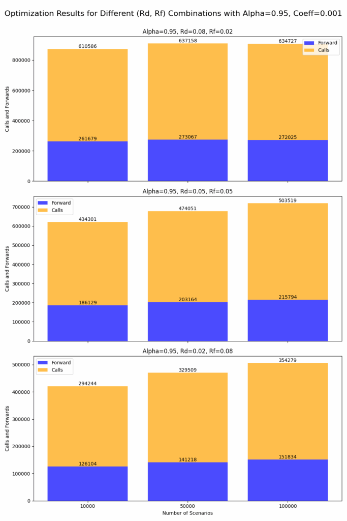
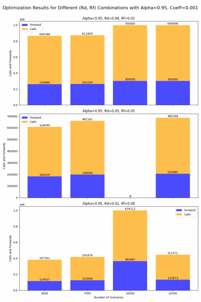
The first set of experiments compares the basic CVaR model, the mixed model, and the distributionally-robust mixed (DRO-mix) model under three market regimes: (R_d, R_f) \in {(0.08,0.02), (0.05,0.05), (0.02,0.08)}, representing strong, neutral, and weak domestic-currency environments.

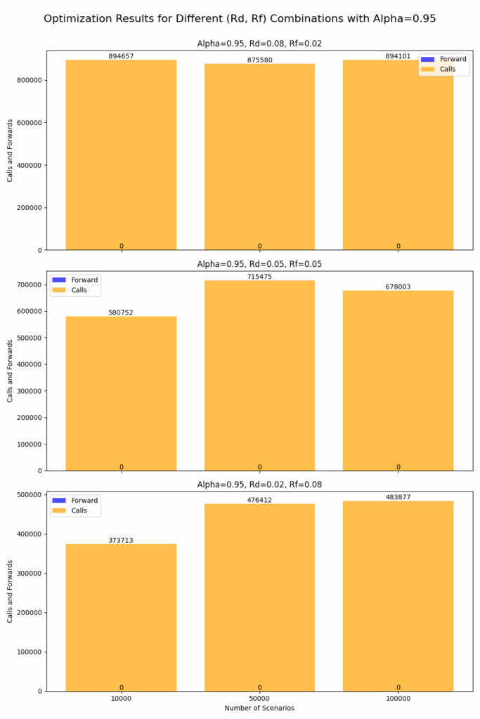
In the basic model, the optimizer almost always selects call options only, as shown in the image on the left.
Forwards are rarely used because they cap potential upside.
This yields a hedge that is profitable when the spot moves favorably but highly sensitive to tail outcomes and volatility spikes.

The mixed model introduces a penalty term \lambda(\theta^+ + \theta^-) that enforces balance between forwards and options.
As seen in the middle image., even a small \lambda (e.g., 0.001) diversifies the hedge, while higher penalties generate more symmetric forward-option mixes that remain stable across all interest-rate regimes.

Finally, the DRO-mixed model extends this formulation by adding an inner maximization over an ambiguity set of probability distributions.
This means the hedge is optimized against the worst-case plausible scenario distribution rather than a single estimated one.
In practice, the effect is visible in the image on the right: the forward exposure increases slightly compared to the standard mixed model, reflecting a more conservative stance.
This model sacrifices some expected profit to achieve greater robustness to estimation error, a critical feature in FX risk management where historical scenario probabilities are highly uncertain.

Performance across Scenarios and Model Complexity

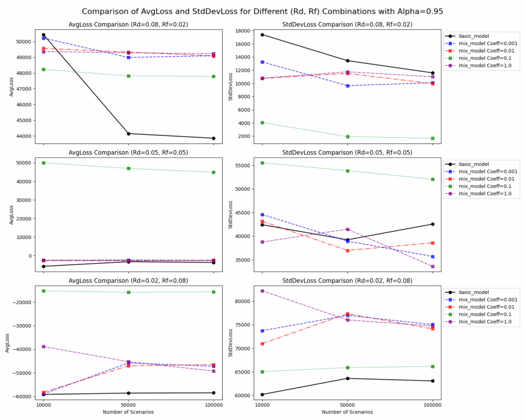
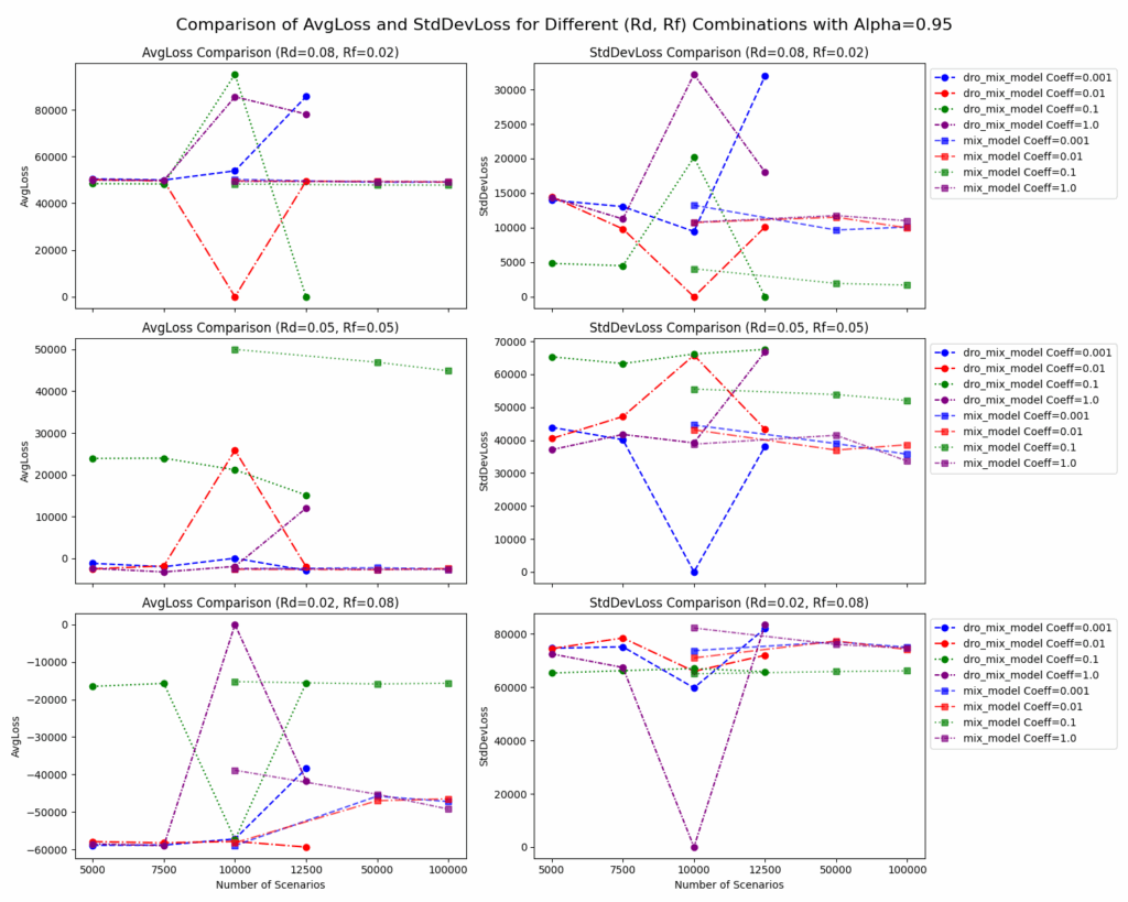
These two figures summarize the average loss and loss volatility (standard deviation) of all models under the same confidence level \alpha = 0.95, across different FX rate regimes and increasing numbers of Monte Carlo scenarios.summarize how the models behave as the number of simulated scenarios increases.
Each point in these plots corresponds to a Monte Carlo estimate of average loss and standard deviation of loss under a given number of scenarios.

Each row corresponds to a different macro setup:

• Top row: R_d = 0.08, R_f = 0.02 → strong domestic currency (EUR strength).
• Middle row: R_d = 0.05, R_f = 0.05 → neutral rate parity.
• Bottom row: R_d = 0.02, R_f = 0.08 → weak domestic currency (EUR depreciation).

Each column represents:

• Left: Average portfolio loss (expected outcome under scenarios).
• Right: Standard deviation of the loss (a proxy for residual risk/volatility).

The figure on the left compares the Basic CVaR model (black line) with several Mixed model configurations (colored dashed lines) using different penalty coefficients \lambda \in {0.001, 0.01, 0.1, 1.0}.

Key patterns:

• The Basic model achieves lower average loss in favorable scenarios but suffers higher variability, showing poor stability when scenario sampling changes.
• As \lambda increases, the Mixed model transitions from risk-seeking to risk-balancing behavior: average losses converge and volatility (StdDevLoss) declines significantly.
• The best trade-off is typically achieved at \lambda = 0.01 or 0.1, where tail risk is minimized without over-hedging.
• In weak EUR environments (bottom row), the penalty stabilizes the results: losses stay centered near zero, while the Basic model shows large swings as the number of scenarios grows.

This confirms that adding a small structural constraint between forwards and options enhances both robustness and generalization.

The second figure introduces Distributional Robustness (DRO) into the same framework.
Each line now compares DRO-Mixed models (dotted lines with circular markers) to the standard Mixed models (dashed lines with square markers).

Interpretation:

• DRO introduces an inner maximization over a probability set, forcing the optimizer to perform well under worst-case distributions.
• As a result, average losses are slightly higher (a conservative bias), but standard deviation decreases across all (Rd, Rf) regimes.
• The difference is particularly visible in volatile regimes, for instance, in the top-right subplot (R_d = 0.08, R_f = 0.02), DRO models maintain stable loss variance even when the number of scenarios changes.
• Models with moderate penalty (\lambda = 0.01) consistently show the smoothest trade-off between robustness and efficiency.

Overall, the DRO-Mixed formulation (right figure) demonstrates how combining moment-based ambiguity sets with structural portfolio balance produces hedges that are less sensitive to data uncertainty and sampling noise, a crucial property in real FX risk management, where scenario probabilities are inherently uncertain.

Tail Behavior and VaR–CVaR Consistency

To understand how these optimizations affect extreme losses, each model’s solution was re-simulated under 100,000 random FX outcomes. The resulting loss distributions are shown in the set of histograms under output/model/loss_distribution on GitHub. Each plot highlights the average loss (green line) and the Value-at-Risk (red line).
Losses are expressed as positive magnitudes (higher = worse outcome) unless otherwise indicated.
The contrast between them illustrates how CVaR accounts for the tail mass beyond the VaR threshold.

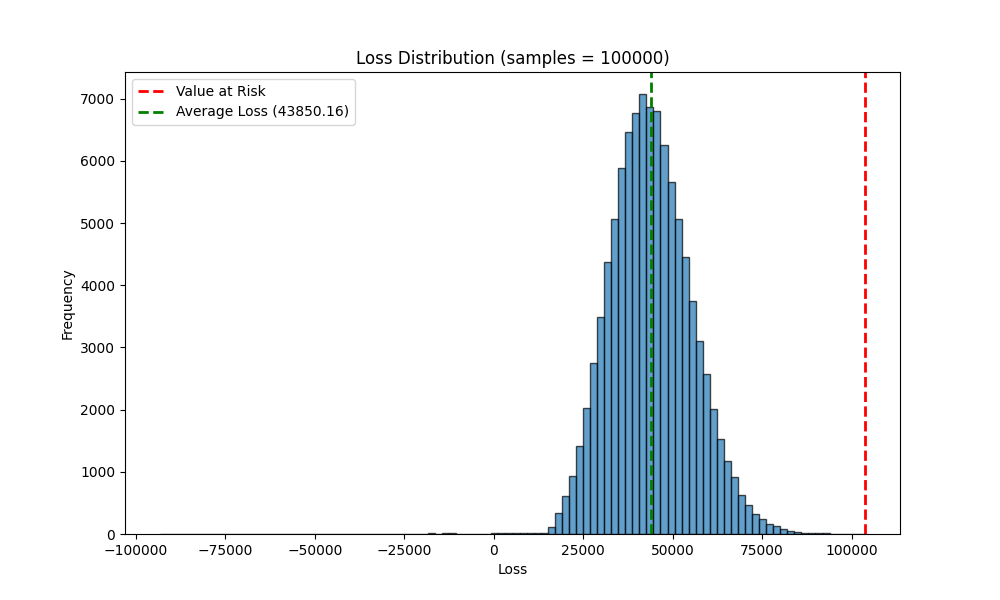
The loss distribution under the basic model shows a pronounced right skew with wide tails. Most outcomes cluster near moderate losses, but large negative events remain relatively frequent, leading to a heavy-tailed profile. The average loss is around 43,850, while the Value at Risk (VaR) line marks the extreme quantile of the tail, indicating substantial exposure to adverse scenarios.

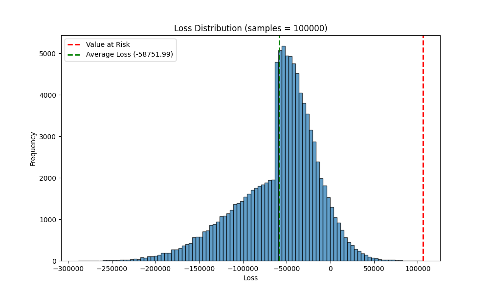
In the mixed model, the loss distribution becomes more symmetric and concentrated. Both tails are significantly compressed compared to the basic model, and the average loss (about –58,752) shifts closer to zero, reflecting improved hedging efficiency. The overall risk profile is smoother, with reduced occurrence of extreme losses.

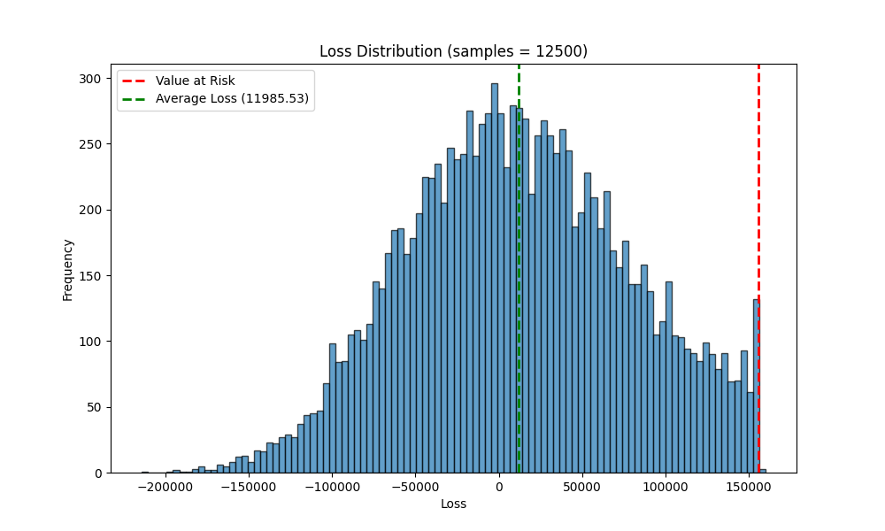
This smaller-sample simulation of the mixed model preserves the general pattern: a narrower, bell-shaped loss distribution with reduced volatility. Despite fewer samples, the mean remains close to 11,986, confirming the model’s robustness and stability under stochastic sampling variations.

These results demonstrate that penalizing deviation between forwards and options, and then adding distributional robustness, effectively stabilizes the risk profile of the hedge even in the presence of model uncertainty.

Sensitivity to Confidence Level α

Increasing the confidence level \alpha from 0.68 to 0.95 and 0.99 progressively shifts the optimizer’s focus from average performance to tail protection.
In the histograms for α=0.68 losses are nearly symmetric, indicating mild risk aversion.
By α=0.99, the optimizer prioritizes the worst scenarios, leading to a heavier allocation in forwards and a visibly truncated loss tail.

Computational Trade-Offs

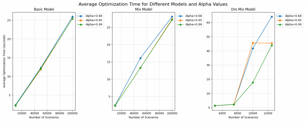
Finally, the image above compares the average runtime of the three optimization formulations.
The basic and mixed models scale linearly with the number of scenarios, while the DRO model exhibits a sharp increase, up to ~60 s for 12,000 samples.
This highlights the cost of robustness: stronger tail control and distributional safety come at the expense of additional constraints and decision variables.

Key Takeaways

• Forward–option balance: Introducing a small \lambda penalty creates smoother, more diversified hedges that dominate the pure CVaR formulation in both mean and variance of loss.
• Distributional robustness: The DRO extension mitigates model-risk sensitivity by hedging against uncertainty in the scenario probabilities.
• Tail risk control: CVaR-based optimization effectively limits catastrophic outcomes, as visible from the narrowing tails in the simulated loss histograms.
• Computation vs stability: The more robust the model, the higher the computational cost, but the gain in stability is significant for real-world risk management.

Closing Remarks

This project shows how quantitative optimization can move beyond textbook hedging.
By embedding modern risk measures (VaR, CVaR) and robust optimization ideas into an executable Python + Gurobi framework, it becomes possible to design hedges that are statistically reliable and financially interpretable.
The final engine, available on GitHub as RiskManagement, can serve as a reusable foundation for scenario-based risk analysis in currencies, commodities, or even multi-asset portfolios.