Abstract

This project explores the prediction of financial market volatility using both classical machine-learning and deep-learning approaches.
I began with a Random Forest baseline model based on engineered technical indicators and progressively developed two recurrent architectures: a univariate and a multivariate Long Short-Term Memory (LSTM) network to capture sequential dependencies in financial time series.

The models were trained on daily data from Apple (AAPL) spanning 2010–2022, using realized volatility as the target variable.
Results demonstrate a progressive improvement in predictive performance, with Mean Absolute Error (MAE) decreasing from 0.0878 (Random Forest) to 0.0517 (multivariate LSTM).

Introduction

This work was developed as part of the Machine Learning and Deep Learning course in my Quantitative Finance Master’s program at Collegio Carlo Alberto.
The goal was to understand how data-driven methods can improve the forecasting of stock market volatility, a central variable for risk management, derivatives pricing, and portfolio allocation.

Traditional econometric models such as GARCH or HAR capture volatility clustering but assume linear and stationary relationships.
Machine learning algorithms like Random Forests, in turn, handle non-linearities but treat each day as an independent sample, missing the sequential nature of financial data.
Deep learning, especially LSTM architectures, offers a middle ground: they can model both non-linear and temporal dependencies, potentially capturing latent “regimes” of volatility persistence.

This study follows the structure proposed by Chatterjee et al. (2022) in IEEE MysuruCon, extending it through richer feature engineering, deeper interpretability, and multi-asset learning.

Data and Feature Engineering

Data Source

Daily OHLC data for Apple (AAPL) were collected via the Yahoo Finance API for the period 2010–2022.
In the multivariate extension, additional stock series were included to represent cross-asset market information (e.g., large-cap peers and sector indices).

Feature Construction

Features were engineered using the pandas-ta library, combining both short-term and long-term indicators of realized volatility, momentum, and trend strength.
The goal was to design a compact yet informative feature set capable of representing market micro-dynamics that typically precede volatility shifts.

• Average True Range (ATR): computed over multiple rolling windows (5, 14, 21, 63 days).
  ATR measures the average magnitude of daily price movements, taking into account both intraday range and overnight gaps.
  Short windows (e.g., ATR₅) react quickly to sudden shocks, while longer windows (ATR₂₁, ATR₆₃) capture persistent volatility regimes.
  Ratios such as ATR_ratio_k = ATRₖ / ATR₆₃ were also introduced to express relative deviations from long-term volatility levels.
• Historical Volatility (HV): the realized standard deviation of log-returns over a fixed look-back period:
  HV_n = \sqrt{\frac{1}{n}\sum_{i=1}^{n}(r_{t-i}-\bar{r})^2}
  Windows of 10, 21, and 63 days were selected to align with typical short, monthly, and quarterly horizons in risk management.
  These indicators quantify the statistical dispersion of returns and serve as direct approximations of realized risk.
• Chaikin Volatility (CHV): a momentum-style measure derived from the Accumulation/Distribution Line (ADL).
  It reflects the rate of change of the trading range (high–low) over a given window.
  CHV provides insight into market pressure: increasing values often precede trend reversals or regime shifts, as they signal widening ranges due to rising uncertainty or liquidity imbalance.
• True Range Rate-of-Change (TR_ROC): captures the velocity of change in the true range.
  It helps identify the acceleration or deceleration of volatility.
  For example, a positive TR_ROC indicates expanding intraday ranges, an early warning for volatility bursts.
• Lagged Volatility and Return Terms: to embed temporal dependencies, several lagged versions of both realized volatility and daily log-returns were included (e.g., Vol_lag1, Ret_lag1, Ret_lag5).
  These lags allow non-recurrent models such as Random Forests to access past information explicitly, while also improving feature diversity for the LSTM when concatenated with recurrent states.

Together, these indicators form a multi-scale representation of market dynamics.
Short-term features (ATR₅, HV₁₀) provide responsiveness to sudden shocks, while long-term components (ATR₆₃, HV₆₃) stabilize predictions by encoding slow-moving volatility regimes.

The target variable is the next-day realized volatility, computed as the rolling 21-day standard deviation of log returns:

r_t = \ln\frac{P_t}{P_{t-1}}, \qquad \sigma_t = \sqrt{\frac{1}{n}\sum_{i=1}^{n}(r_{t-i} – \bar{r})^2}

Data were normalized using Min-Max scaling, and train/test splits were chronological to avoid look-ahead bias.

Methodology

Random Forest Baseline

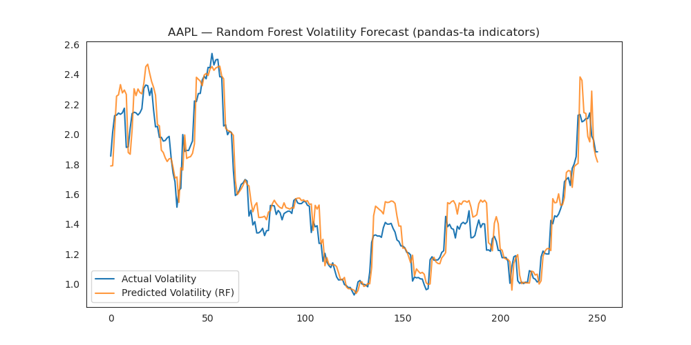
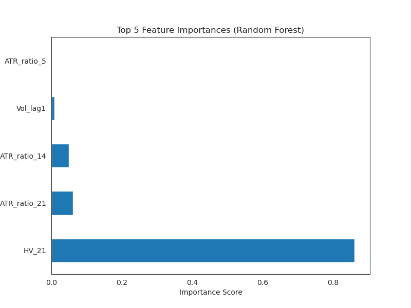
The baseline model uses a Random Forest regressor with 500 trees and maximum depth of 10.
The feature importance plot shows that HV_21 dominates the model, accounting for more than 80% of the predictive contribution, while short-term ATR ratios add minor incremental value.
This confirms the persistence of recent volatility as the strongest short-term predictor.
However, the model remains static and fails to adapt quickly during structural volatility shifts.

Univariate LSTM

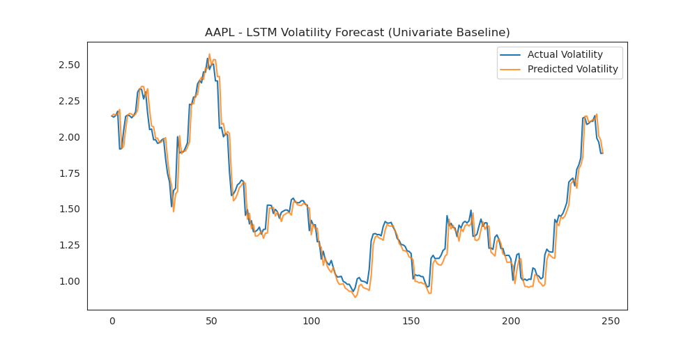
The next step was to implement a stacked LSTM network that learns volatility patterns directly from sequences of past values.
This model serves as the base deep-learning architecture before extending to the multivariate setup.
It is designed to predict the 21-day rolling realized volatility of a single stock (AAPL) using its historical time series.

Configuration:

• Sequence length: 5
• Learning rate: 1×10⁻³
• Epochs: 100
• Optimizer: Adam
• Loss: L1 (Mean Absolute Error)
• Batch size: 256

The model consists of three LSTM layers followed by a dense output neuron.
The choice of an L1 loss function reflects the focus on median error robustness, an important property when working with heavy-tailed financial series.
The relatively short sequence length of 5 trading days was chosen to prioritize local temporal dependencies without over-smoothing regime changes.

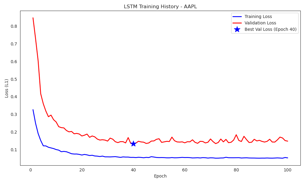
During training, both the training and validation losses stabilized around epoch 40, achieving MAE = 0.0579 and RMSE = 0.0861 on the test set.
The learning curve indicates healthy generalization, with validation error converging smoothly toward the training loss.
The forecast aligns closely with realized volatility, successfully capturing both amplitude and persistence of high-volatility phases.

Multivariate LSTM

To further enhance predictive power, the LSTM architecture was extended to a multivariate setting, where the model receives as input not only Apple’s own historical data but also returns and volatilities from multiple assets.
This richer input space enables the network to learn inter-asset dependencies and market-wide volatility transmission effects, a crucial aspect in financial systems where volatility shocks often propagate across assets and indices.

The model was designed to predict Apple’s next-day realized volatility from a feature matrix including AAPL, MSFT, NVDA, S&P 500 (^GSPC), and VIX daily returns and rolling volatilities.
This effectively transforms the problem from a single-variable memory task into a multivariate temporal modeling problem.

Configuration:

• Sequence length: 10
• Learning rate: 1×10⁻⁴
• Epochs: 400
• Optimizer: Adam
• Loss: L1 (Mean Absolute Error)
• Batch size: 256

The larger sequence length and lower learning rate reflect the higher dimensionality of the input and the smoother training dynamics required for multi-asset data.
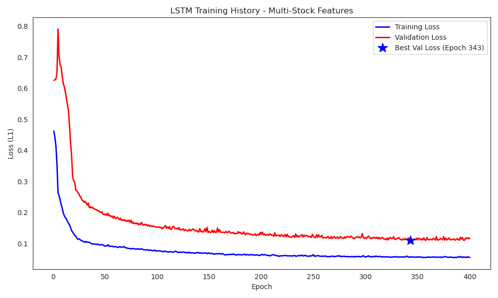
Training converged gradually, reaching optimal validation loss around epoch 343.
On the test set, the model achieved MAE = 0.0517 and RMSE = 0.0777, marking the best performance among all tested approaches.

The training and validation curves exhibit stable learning without divergence, confirming that the model generalizes well across market conditions.
Compared to the univariate version, the multivariate LSTM produces smoother volatility trajectories and adapts more effectively to regime transitions, particularly during high-volatility periods.

Interpretability and Internal Representations

Understanding how deep networks represent volatility dynamics was one of the most interesting parts of this work.

Activation Analysis

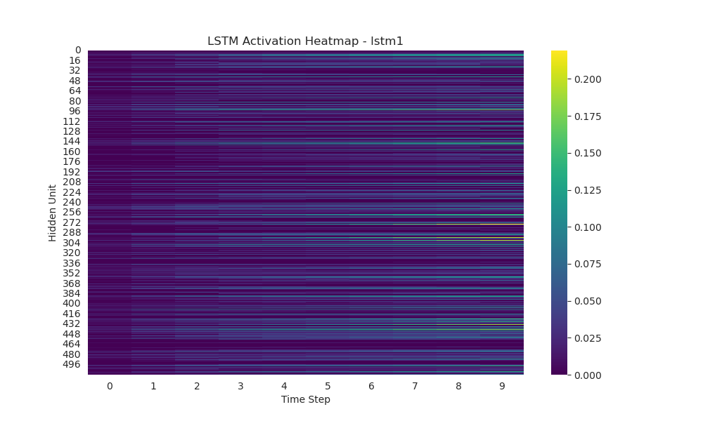
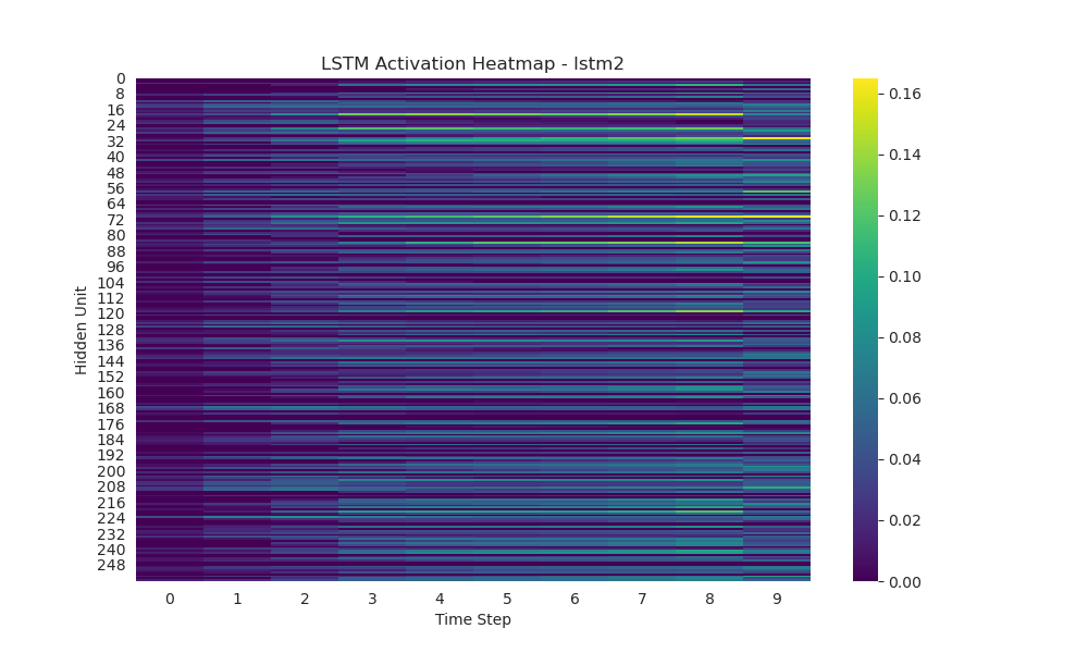
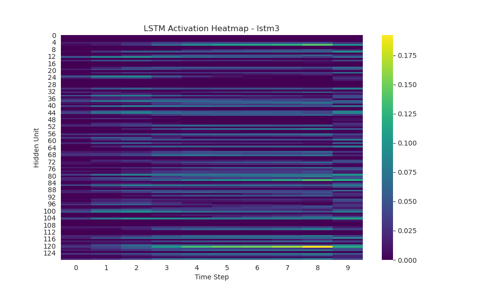
Activation heatmaps across the three LSTM layers illustrate how information is progressively filtered and abstracted through the network.

• The first layer reacts broadly to short-term fluctuations, showing sparse and scattered activations that mirror high-frequency noise in market data.
• The intermediate layer begins to focus on more coherent temporal structures, selectively amplifying sequences that precede volatility shifts.
• By the final layer, the activation patterns become sharply localized, reflecting the network’s ability to encode specific volatility regimes rather than individual price movements.

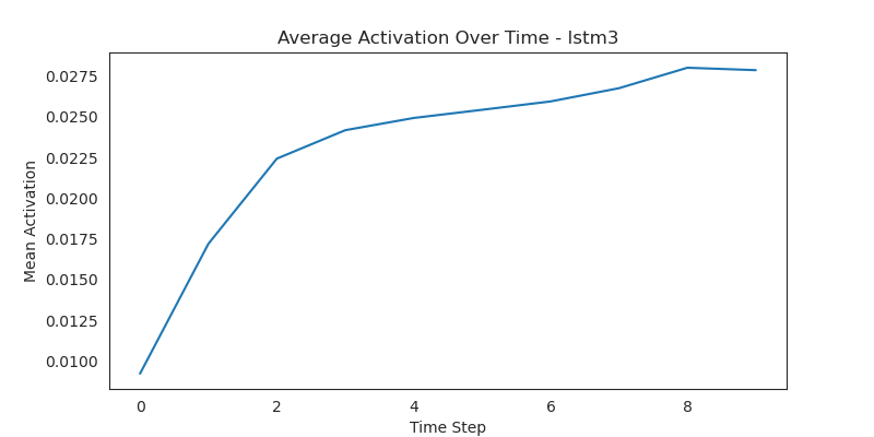
The average activation curve confirms this evolution: activation intensity increases toward the end of each sequence, indicating that recent timesteps carry greater predictive weight.
This behavior aligns with financial intuition, the most recent market conditions typically dominate short-term volatility forecasts.

High vs Low Volatility Behavior

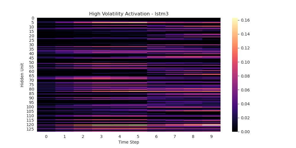
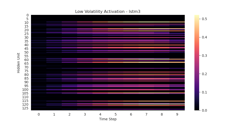
By isolating samples from high- and low-volatility periods, I observed that the network engages different subsets of neurons across its final LSTM layer.
During high-volatility states, activations become sharply concentrated within a few units, suggesting that the model focuses its internal dynamics on a limited set of features highly sensitive to market stress.
In contrast, low-volatility phases display broader and more evenly distributed activations, reflecting a stable regime where no single input dominates the forecast.
This clear functional separation indicates that the network has developed an implicit internal encoding of volatility regimes, dynamically reallocating its representational capacity based on market conditions.

Latent Space Visualization

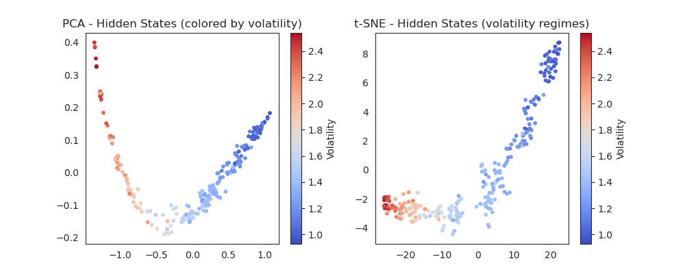
Applying Principal Component Analysis (PCA) and t-distributed Stochastic Neighbor Embedding (t-SNE) to the hidden-state representations reveals that the network embeds volatility dynamics into a continuous low-dimensional manifold.
While PCA performs a linear projection to highlight the main axes of variance, t-SNE is a non-linear dimensionality reduction algorithm that preserves local relationships between points, meaning that data points close in the original high-dimensional space remain close in the 2D projection.
This makes t-SNE particularly suited for visualizing latent structures learned by deep models.

In this representation, samples form smooth trajectories that transition across low, mid, and high-volatility regimes, showing how the LSTM internally organizes market behavior.
Such clustering indicates that the model captures not just short-term fluctuations, but also the structural patterns underlying regime shifts, effectively constructing a latent map of market dynamics.

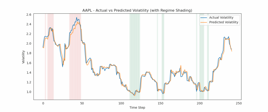
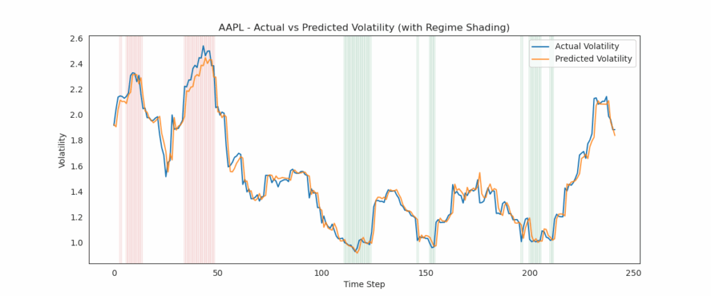
The comparison between actual and predicted volatility demonstrates the model’s ability to closely follow real market fluctuations.
Shaded areas indicate distinct volatility regimes, as inferred from the hidden-state clustering: red bands mark turbulent, high-volatility periods, while green regions correspond to stable, low-volatility phases.
The LSTM effectively adapts across these transitions, maintaining smooth predictions even during rapid regime shifts.
This alignment between predicted and observed volatility, particularly around turning points, suggests that the model not only tracks realized risk, but also anticipates structural changes in market behavior, reinforcing the interpretability of the learned latent representations.

Integrated Gradients

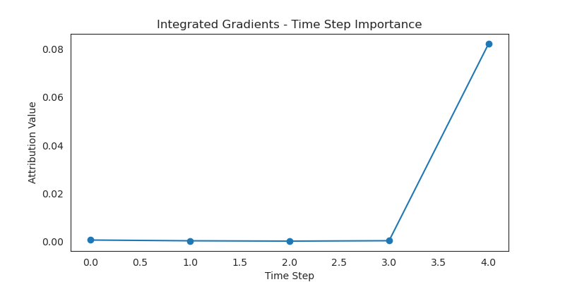
Using the Captum library, I applied the Integrated Gradients (IG) method to measure how much each timestep contributes to the model’s output.
Integrated Gradients is an explainability technique for neural networks that attributes the prediction to its input features by integrating the model’s gradients along a straight path from a baseline input (often all zeros) to the actual input.
Intuitively, it quantifies how the prediction changes as the input gradually moves from a neutral state to its real value, providing a mathematically principled measure of feature importance.

In this context, IG reveals that the final timestep has by far the largest attribution value (around 0.08), meaning that the model’s volatility forecast relies heavily on the most recent observations.
This confirms that the LSTM captures the temporal dependency structure typical of financial markets, where the latest price and volatility movements dominate short-term risk expectations.

Results Summary

Model	MAE	RMSE	Key Insight
Random Forest	0.0878	0.1153	Non-sequential baseline; heavily reliant on HV_21
LSTM (Univariate)	0.0579	0.0861	Captures volatility memory; learns smooth transitions
LSTM (Multivariate)	0.0517	0.0777	Best performance; integrates cross-asset dependencies

The performance improvement from Random Forest to multivariate LSTM represents a 41% reduction in MAE, confirming that sequential and multi-asset modeling significantly enhances volatility predictability.
The interpretability analyses further show that deep networks, while complex, can yield meaningful insights into market structure when carefully examined.

Discussion

This progression from Random Forest to univariate and then multivariate LSTM highlights how different modeling assumptions capture distinct aspects of financial volatility:

• Random Forest leverages engineered features and achieves solid baseline performance but cannot model temporal causality.
• Univariate LSTM learns sequential dependencies, outperforming RF by roughly one-third, though limited by its single-asset scope.
• Multivariate LSTM generalizes better by capturing shared volatility shocks and co-movements between assets.

The internal representations observed through PCA and activation heatmaps suggest that LSTMs naturally encode regime structures without explicit labels or supervision.
This emergent organization provides an intuitive interpretation: the network learns an internal “volatility map” where states evolve smoothly across market phases.

However, challenges remain:

• Limited interpretability relative to traditional econometric frameworks.
• Potential overfitting due to high model flexibility.
• Absence of exogenous signals (macroeconomic or sentiment-based).

These aspects point toward hybrid or transformer-based models as promising future directions.

Conclusions

Through this project, I learned how to move from feature-based machine learning to sequence-based deep learning, and how to interpret what deep models “see” when forecasting volatility.
I realized that performance improvement alone is not the main outcome, it is the understanding of how models process information that really adds value.

Building and analyzing these models improved my understanding on:

• The importance of robust preprocessing and feature scaling in time-series tasks.
• How hyperparameter tuning (e.g., sequence length, learning rate) shapes convergence.
• How activation and attribution analysis can transform black-box networks into interpretable systems.
• That latent-space visualizations provide an elegant way to observe how neural networks perceive market regimes.

From a broader perspective, this work deepened my intuition for volatility dynamics and reinforced the idea that interpretability is as valuable as prediction accuracy in quantitative finance.

References

Chatterjee, A., Bhowmick, H., & Sen, J. (2022). Stock Volatility Prediction using Time Series and Deep Learning Approach. IEEE MysuruCon 2022.
DOI: 10.1109/MysuruCon55714.2022.9972559